Solving Riddle of Code Efficiency: Understanding Time Complexity with

Introduction:

In the coding world, we often want to know how fast or slow our code is, especially when dealing with large amounts of data. Big-O notation is like a cheat sheet that helps us understand and compare the efficiency of different code solutions.

What's Big-O Notation?

Big-O notation is a fancy way of saying, "Hey, how does the speed of our code change when we throw more stuff at it?" It's like predicting how your favorite game might slow down when there are too many players. In one line it's like comparing the efficiency of different code solutions.

Why Do We Care About Time Complexity?

Imagine we have a magic recipe to solve a problem. Time complexity helps us figure out if our recipe is great for a few friends (small problems) or a big party (huge problems). It helps us choose the right solution based on how much work our computer needs to do. It's like measuring the capability of your code on a broad factor.

Asymptotic notation simplification

Imagine you have an algorithm, and someone tells you its time complexity is T(n)=3n^2+2n+1, where n is the size of the input.

Now, we want to make this simpler to understand:

Find the Big Part:
- Look at the terms and find the one that grows the fastest. In our case, it's 3*n^*2.
Ignore the Smaller Parts:
- Forget about the terms that don't grow as fast. Here, 2n and 1 are not as important.

T(n) simplifies to O(n2)

We don't worry about the exact number (3) because we care more about how things grow.

So, instead of saying T(n)=3n2+2n+1, we can simply say the time complexity is O(*n^*2). This way, we express how the algorithm's performance changes as the input gets larger in a much simpler way. There's a big mathematical description about this topic but we skip the boring part.

Big-O Notation: Code Example

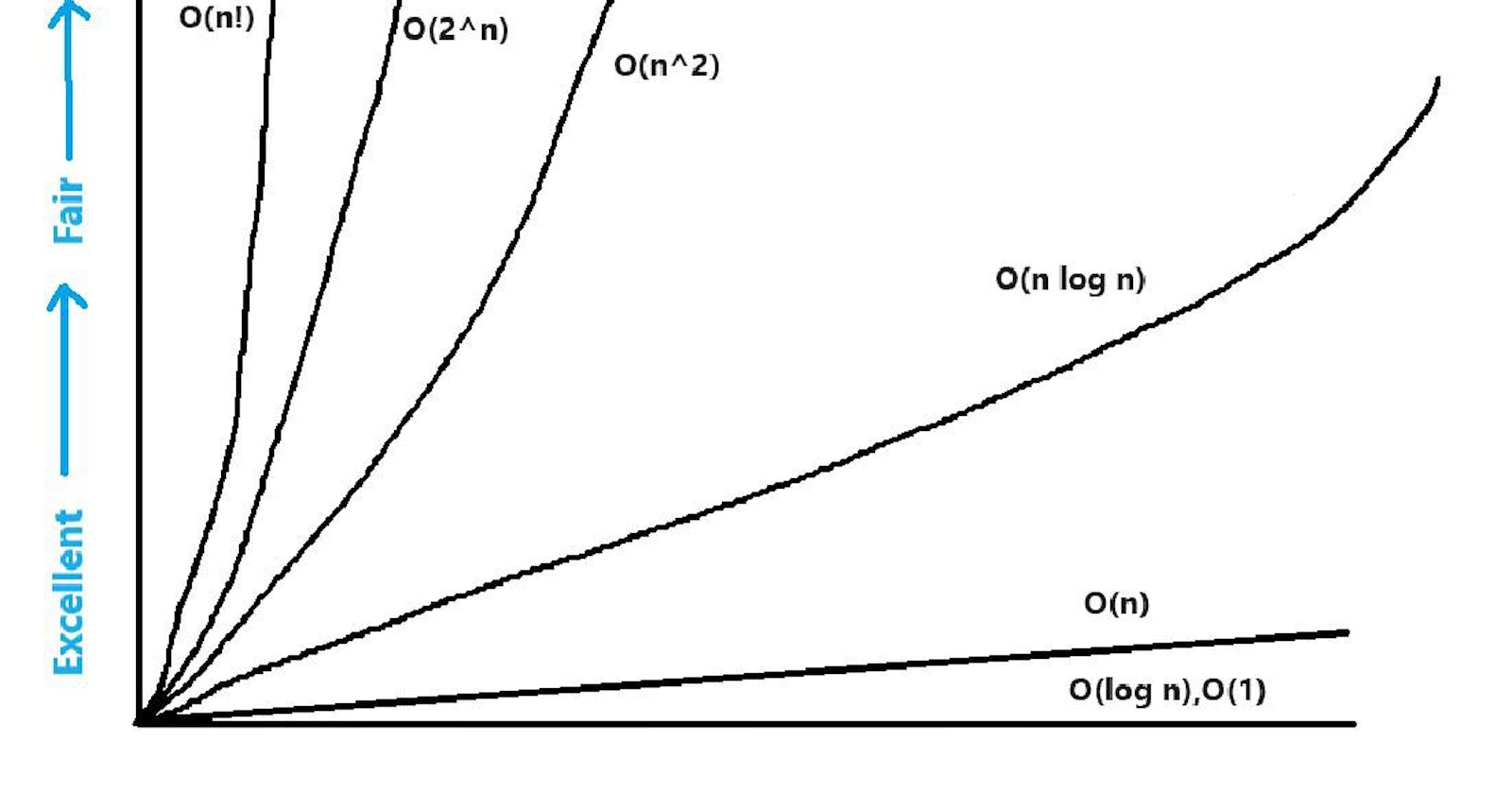
O(1) - Constant Time:
- Example: Accessing an element in an array using its index.
- Visual Representation: A flat line because it takes the same amount of time regardless of the input size.

O(log n) - Logarithmic Time:

Example: Binary search in a sorted array.
Visual Representation: A gradually increasing curve, showing that the algorithm becomes less sensitive to input size as it grows.

    def binary_search(arr, target):
        """
        Binary search implementation with logarithmic time complexity.

        Parameters:
        - arr: A sorted list of elements.
        - target: The element to search for in the list.

        Returns:
        - index: The index of the target element if found, otherwise -1.
        """
        low, high = 0, len(arr) - 1

        while low <= high:
            mid = (low + high) // 2  # Calculate the middle index

            if arr[mid] == target:
                return mid  # Target found, return the index
            elif arr[mid] < target:
                low = mid + 1  # Discard the left half
            else:
                high = mid - 1  # Discard the right half

        return -1  # Target not found in the list

    # Example Usage:
    sorted_list = [1, 2, 3, 4, 5, 6, 7, 8, 9, 10]
    target_element = 7

    result = binary_search(sorted_list, target_element)
    if result != -1:
        print(f"Element {target_element} found at index {result}.")
    else:
        print(f"Element {target_element} not found in the list.")

O(n) - Linear Time:

Example: Finding the maximum element in an unsorted array by scanning each element once.
Visual Representation: A straight line, indicating a direct relationship between the input size and the algorithm's performance.

  def linear_search(arr, target):
      """
      Linear search implementation with linear time complexity.

      Parameters:
      - arr: A list of elements.
      - target: The element to search for in the list.

      Returns:
      - index: The index of the target element if found, otherwise -1.
      """
      for i in range(len(arr)):
          if arr[i] == target:
              return i  # Target found, return the index

      return -1  # Target not found in the list

  # Example Usage:
  example_list = [3, 7, 1, 9, 4, 6, 8, 2, 5]
  target_element = 6

  result = linear_search(example_list, target_element)
  if result != -1:
      print(f"Element {target_element} found at index {result}.")
  else:
      print(f"Element {target_element} not found in the list.")

O(n log n) - Linearithmic Time:
- Example: Many efficient sorting algorithms like Merge Sort and Heap Sort.
- Visual Representation: A curve that grows faster than linear but not as fast as quadratic. It's often more efficient than O(n^2) for large datasets.
- Merge Sort implementation with linearithmic time complexity.
O(n^2) - Quadratic Time:
- Example: Nested loops to compare all pairs of elements in an array (Bubble Sort).
- Visual Representation: An upward-sloping curve, indicating that the algorithm's performance grows quadratically with the input size.
O(2^n) - Exponential Time:
- Example: Brute-force solutions for problems like the Traveling Salesman Problem.
- Visual Representation: A very steep curve, showing a significant increase in time as the input size grows. This is generally less efficient and should be avoided for large datasets.

Wrapping Up

Big-O notation is our secret code to talk about how fast our code can handle different amounts of work. By keeping things simple and visualizing with graphs, we become coding superheroes, ready to tackle any challenge efficiently!

Refat's Blog